Descriptive statistics

Measures of central tendency

• Three main measures of central tendency: Mean (average), median (middle value), and mode (most frequent value)

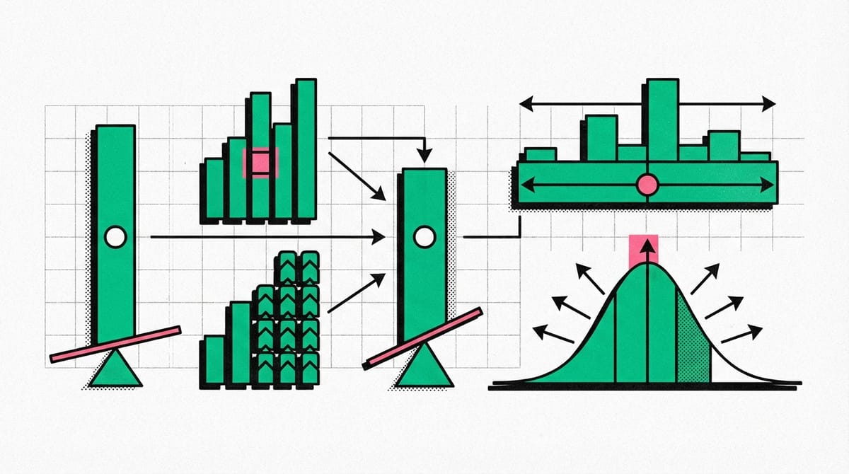
First, I want to know the center of my dataset, then I want to know how other values are distributed relative to the center. Measuring the center and spread of a dataset helps me quickly understand its overall structure and decide which parts I want to explore in more detail.

• Mean calculation: Sum of all values divided by the total number of values
• Median identification: Middle value when data is arranged in order; average of two middle values for even-numbered datasets

The mean and median work better for different types of data. If your dataset has outliers, the median is usually a better measure of center. If there are no outliers, the mean usually works well.

For example, imagine you want to buy a house in a specific neighborhood. You tour ten homes in the area to get an idea of the average price. The first nine homes have a price of $100,000. The tenth home costs a million dollars. This is an outlier that pulls up the average. If you add all the home prices and divide by 10, you'll find that the mean or average price is $190,000. The mean doesn't give you a good representation of the typical home value in this neighborhood. In fact, only one home out of ten costs more than $100,000. The median home price is $100,000. The median gives you a much better idea of the typical home value in this neighborhood. Whether you use the mean or median depends on the specific dataset you're working with and what insights you want to gain from your data.

• Mode characteristics: Can have no mode, one mode, or multiple modes; particularly useful for categorical data
• Choosing the right measure:
  • Use median when dataset contains outliers
  • Use mean when data is relatively uniform without outliers
  • Use mode for categorical data analysis
• Purpose: These measures help quickly understand dataset structure and guide further analysis steps.

Measures of central tendency: The mean, the median, and the mode

• The mean is best used when data has no significant outliers and represents a typical average value.
• The median is more reliable when dealing with datasets that contain outliers, as it's less sensitive to extreme values.
• The mode is particularly useful for categorical data and shows the most frequent occurrence in a dataset.
• When analyzing data, it's important to consider which measure of central tendency best represents your specific dataset.
• Using multiple measures of central tendency together can provide a more complete understanding of your data's distribution.

Measures of dispersion

• Measures of dispersion help understand how spread out data values are from the center
• Two main measures of dispersion are:
  • Range: Difference between largest and smallest values
  • Standard deviation: Average distance of data points from the mean
• Larger standard deviation indicates data points are more spread out from the mean
• Standard deviation calculation involves 5 steps:
  • Find the mean
  • Calculate distance to mean for each value
  • Square the distances
  • Sum squares and divide by (n-1)
  • Take the square root
• Understanding dispersion is crucial for:
  • Making accurate predictions
  • Interpreting data variation
  • Real-world applications like weather forecasting

Now let's look at an example of how standard deviation is useful in everyday life. Meteorologists use standard deviation for weather forecasting to understand how much variation exists in daily temperatures in different locations and to make more accurate weather predictions. Imagine two meteorologists working in two different cities, City A and City B. During March, City A has a mean temperature of 66 degrees Fahrenheit and a standard deviation of three degrees. City B has a mean temperature of 64 degrees Fahrenheit and a standard deviation of 16 degrees. Both cities have similar mean temperatures. In other words, the overall average temperature is about the same, but the standard deviation is much higher in City B. This means there is more daily temperature variation there. The weather can change dramatically from day to day. In City A, the weather is more stable. If the meteorologist in City B predicted the weather based on the mean, they could be off by 16 degrees, which would lead to a lot of unhappy residents. The standard deviation gives the meteorologist a useful measure of variation to consider and a level of confidence in their prediction. A low standard deviation in temperature makes it much easier for the meteorologist in City A to accurately predict daily weather.

Measures of dispersion: Range, Variance, and Standard deviation

• Standard deviation is a fundamental statistical measure that quantifies data spread around the mean
• Three main measures of dispersion are range (simplest), variance (squared differences), and standard deviation (square root of variance)
• A smaller standard deviation indicates data points cluster closer to the mean, while a larger one shows greater spread
• Understanding standard deviation is crucial for:
  • Comparing datasets with similar means but different distributions
  • Making informed decisions about data analysis methods
  • Identifying unusual patterns or outliers in datasets
• In real-world applications, standard deviation helps quantify variability in areas like financial analysis, quality control, and market research
• While computers handle the calculations, understanding the concepts behind standard deviation is essential for proper data interpretation.

Measures of position

• Measures of Position: Help determine the position of values in relation to other values in a dataset
• Percentiles: Show the value below which a percentage of data falls, useful for comparing values across different scoring systems
• Quartiles: Divide data into four equal parts:
  • Q1 (25th percentile): Lower quartile
  • Q2 (50th percentile): Median
  • Q3 (75th percentile): Upper quartile
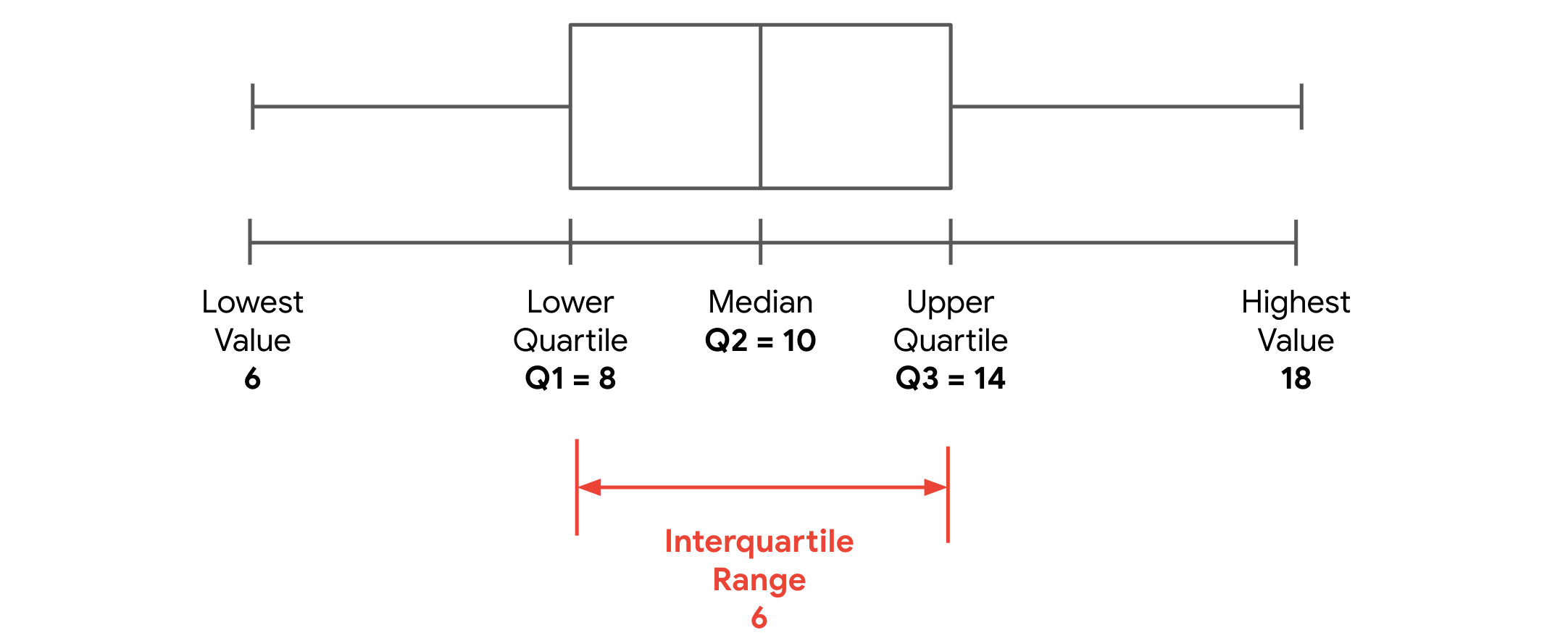
• Interquartile Range (IQR): Measures the spread of the middle 50% of data, calculated as Q3 - Q1

For example, let's say you're a sports team manager. You have data showing how many goals each player on your team scored throughout the season. You want to compare the performance of each player based on goals scored. You can calculate quartiles for your data using the following steps. First, arrange the values from smallest to largest: 11, 12, 14, 18, 22, 23, 27, 33. Second, find the median of your dataset. This is the second quartile, Q2. Since there is an even number of values in the dataset, the median is the average of the two middle values, 18 and 22, making Q2 equal to 20. Third, find the median of the lower half of your dataset. This is the lower quartile, Q1, which equals 13. Finally, find the median of the upper half of your dataset. This is the upper quartile, Q3, which equals 25.

• Five-Number Summary: Provides comprehensive data overview including:
  • Minimum value
  • First quartile (Q1)
  • Median (Q2)
  • Third quartile (Q3)
  • Maximum value
• Box Plot: Visual representation of the five-number summary, showing data distribution and potential outliers.

Measures of position: Percentiles and Quartiles

• Percentiles divide data into 100 equal parts and show the relative position of values in a dataset

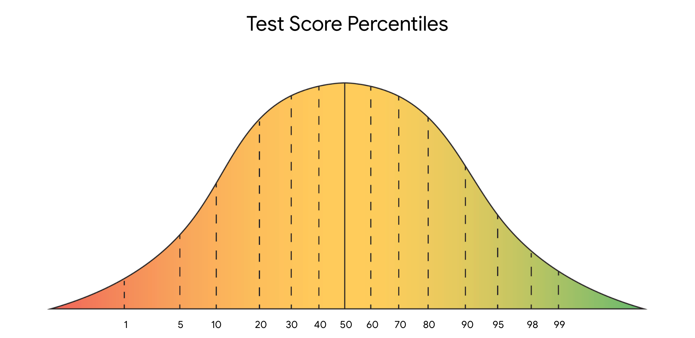
• Quartiles split data into four equal parts (Q1 at 25th percentile, Q2 at 50th percentile, Q3 at 75th percentile)

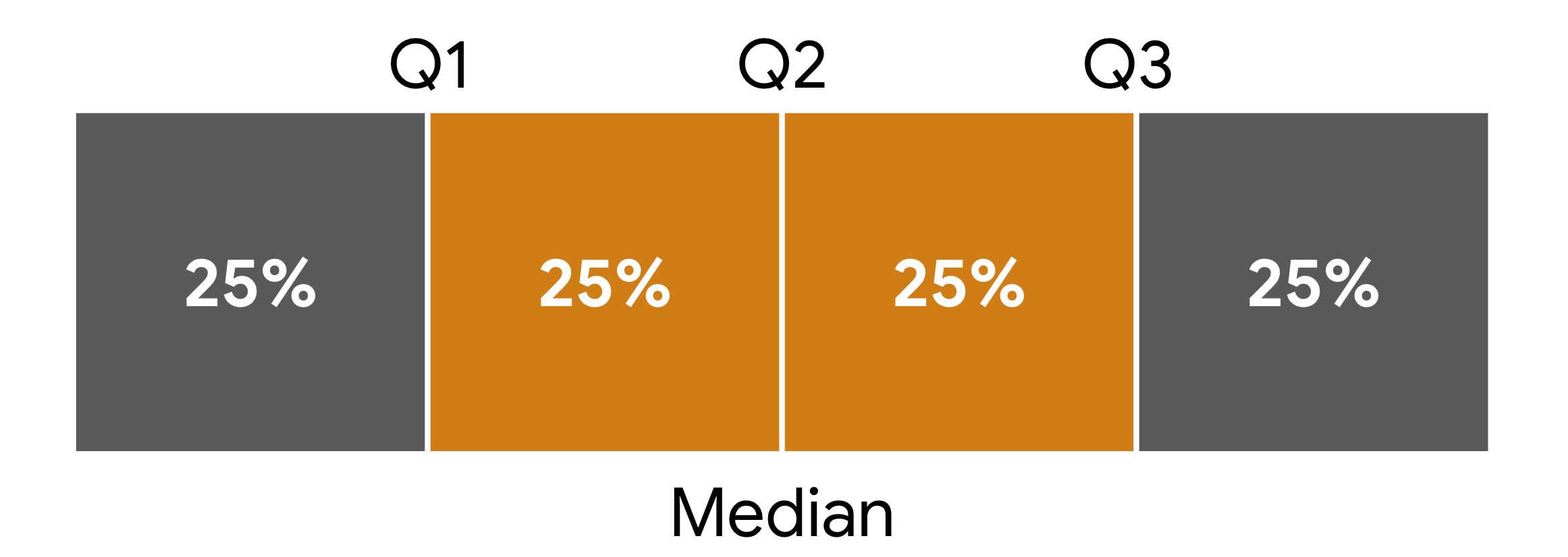
• The Interquartile Range (IQR) measures the spread of the middle 50% of data between Q1 and Q3
• The Five Number Summary (minimum, Q1, median, Q3, maximum) provides a comprehensive overview of data distribution!

• These measures help identify outliers and understand data distribution without being overly sensitive to extreme values.

Statistics as the foundation of Data-driven solutions

• Statistics as Foundation: Statistics combines mathematics with data application, providing essential tools for data professionals.
• Real-world Application: Statistical methods are crucial for generating insights and informing business decisions, especially in A/B testing scenarios.
• Problem Decomposition: Statistics provides tools to break down complex problems and explain data differences systematically.
• Career Development: Having a strong foundation in data analytics and project experience can lead to impactful career opportunities.
• Learning Approach: Success in data analytics requires:
  • Maintaining focus on end goals
  • Taking a step-by-step approach
  • Being resilient when facing challenges

Key Takeaways

• Understanding Central Tendency: Mean, median, and mode provide different perspectives on data center, each suited for specific scenarios.
• Importance of Dispersion: Range and standard deviation reveal how spread out data is, crucial for accurate data interpretation.
• Position Measures: Percentiles and quartiles help understand data distribution and identify outliers effectively.
• Practical Application: Statistical knowledge enables:
  • Better decision-making in data analysis
  • More accurate predictions and forecasting
  • Deeper understanding of data patterns
• Statistical Foundation: Strong statistical knowledge is essential for:
  • Breaking down complex problems
  • Generating meaningful insights
  • Making data-driven business decisions.